Background
In a previous blog post, I discussed the use of application program interfaces (APIs) in R. Specifically, I focused on accessing data from the US Department of Agriculture’s National Agricultural Statistics Survey (NASS) Quick Stats API. Since I wrote that previous blog post in January 2019, several R packages that aid access to the NASS Quick Stats API have come to my attention. With these packages, it’s much easier to access NASS Quick Stats data using R! Specifically, you don’t have to manually explore data availability or manually tidy the data you’ve retrieved, which is what I had to do when determining how to download Quick Stats irrigation data for North Carolina (NC) and when defining variables like nc_irrigated, respectively, in that blog post back in January 2019.
Goals of This Post
The main goal of this blog post is to:
- Use an R package to download and plot Census of Agriculture data from the NASS Quick Stats API.
In addition to Natalie Nelson and Andrew Dau, who I thanked in my previous blog post, I’d like to thank Nicholas Potter at Washington State University for developing the rnassqs package and responding to my questions. Last but not least, I’d like to thank my collaborator Nitin Singh for developing interesting research questions that inspired me to streamline my R code.
Available NASS API Packages
As of the posting date of this blog, there are three main packages to help R users interface with the NASS Quick Stats API:
rnassqs- This package was developed in 2015 by Nicholas Potter at Washington State University and is supported by rOpenSci. To read more about this package, see examples, submit issues/bugs, and contribute to development see here. This package is available on CRAN and you can read the manual here.usdarnass- This package was developed in 2018 by Robert Dinterman at The Ohio State University. To read more about this package, see examples, submit issues/bugs, and contribute to development see here. This package is available on CRAN and you can read the manual here.rnass- This package was developed in 2015 by Emrah Er at Ankara University. To read more about this package, see examples, submit issues/bugs, and contribute to development see here. This package is not available on CRAN, so it would have to be installed via GitHub.
Note: In this post, I’ll present code that uses the rnassqs package only.
Set Up
First let’s load the R libraries that we’ll need to run the code in this blog post.
library(tidycensus)
library(tidyverse)
library(mapview)
The tidycensus, tidyverse, mapview packages should all be familiar from my previous blog post.
The rnassqs package is new to this blog post. You can use it to look up available data on the NASS Quick Stats API and access it. I recommend installing this package from GitHub because you’ll want to use the nassqs_param_values() function which is only available via the package version on GitHub. If you install the package through CRAN using install.packages("rnassqs") this function will not be included. Remember, you only need to install this once but then must call it every time you start a new session.
devtools::install_github("ropensci/rnassqs")Let’s load the NASS API R package.
library(rnassqs)Census API Set Up
As I mentioned in my previous blog post, many APIs require that you have a personal API key to access the data stored within them. To run the code in this post you’ll need to request a Census API key (see instructions below) and a NASS API key (see instructions below). Once you have your own personal API key, you should keep them both in safe and central location. I recommend a text file somewhere memorable on your (password protected) computer.
To request a Census API key, you can go to here and fill in your name and organization. Once you submit the key request, the US Census Bureau will email a Census API key. This key is unique to the name and email you provided, so as I mentioned in the previous paragraph, be sure to keep it in a safe place.
If you’ve never installed your Census API key, you’ll want to install your API key for later using the code below.
CENSUS_API_KEY <- "YOUR API KEY GOES HERE"
census_api_key(CENSUS_API_KEY, install = TRUE)

# The second line of code above will make an entry in your .Renviron file called "CENSUS_API_KEY".
If you’ve already installed your Census API key, you should be good to go, but you can always check to make sure it’s in your R environment using the code below.
# check that it's there
Sys.getenv("CENSUS_API_KEY")
If you want to get tabular and spatial census data using the tidycensus package, you’ll need to run the code below each time you start a new R session. Spatial census data includes, for example, census tract boundaries.
options(tigris_use_cache = TRUE)NASS API Set Up
Be sure to also apply for a NASS API key, which I’ll define in a string called NASS_API_KEY. You can apply for a NASS API key here. As with the Census API key, this is unique to you so be sure to keep it in a safe place.
NASS_API_KEY <- "ADD YOUR NASS API KEY HERE"If you want to save your NASS API key to your R environment, you can use the code below. Setting the NASS API key in your R environment will keep it hidden and accessible only to you. This might be important if you’re planning to pass along your script to someone else…or post it on your blog. ;)
To set the NASS API key your R environment you’ll have to navigate to the (hidden) .Renviron file on your computer. Then you will have to add NASS_API_KEY <- "ADD YOUR NASS API KEY HERE" to that text file. Alternatively, you can also use sys.setenv() as indicated below. See this tutorial and this tutorial. You only need to do this once on your computer.
# add NASS_API_KEY to  your .Renviron file
sys.setenv(NASS_API_KEY <- "ADD YOUR NASS API KEY HERE")
Once you’ve added the NASS API key to your computer’s .Renviron file. You’ll have to run the following code each time you start a new R session. This is because you’ll need to remind R that it has this information available in the .Renviron file.
# load your stored NASS_API_KEY it into your current R session
NASS_API_KEY <- Sys.getenv("NASS_API_KEY")
Before you can make any queries, the rnassqs package requires that you to set your NASS API key using the nassqs_auth() function.
# use your NASS_API_KEY variable (see previous code chunk) to set this as your key
nassqs_auth(key = NASS_API_KEY)

# alternatively if you don't want to store a variable called NASS_API_KEY in your current session, you can run:
# nassqs_auth(key = Sys.getenv("NASS_API_KEY"))
Looking Up Available Data
The first step to building a API query is understanding what parameters you have the ability to request. You can look at a complete list of available parameters using the nassqs_params() function. By saving the output of this to a variable named params_list, you can click on the variable in our RStudio environment and check it out.
params_list <- nassqs_params()

# print out the parameters
params_list
##  [1] "agg_level_desc"        "asd_code"              "asd_desc"
##  [4] "begin_code"            "class_desc"            "commodity_desc"
##  [7] "congr_district_code"   "country_code"          "country_name"
## [10] "county_ansi"           "county_code"           "county_name"
## [13] "CV"                    "domaincat_desc"        "domain_desc"
## [16] "end_code"              "freq_desc"             "group_desc"
## [19] "load_time"             "location_desc"         "prodn_practice_desc"
## [22] "reference_period_desc" "region_desc"           "sector_desc"
## [25] "short_desc"            "state_alpha"           "state_ansi"
## [28] "state_name"            "state_fips_code"       "statisticcat_desc"
## [31] "source_desc"           "unit_desc"             "util_practice_desc"
## [34] "Value"                 "watershed_code"        "watershed_desc"
## [37] "week_ending"           "year"                  "zip_5"
## [40] "format"
There are 40 parameters that can be specified in a query. Looking back at my previous blog post, I was interested in exploring the fraction of irrigated acres of agricultural land in the state of North Carolina over time. To replicate this work using the rnassqs package, I’ll pay attention to 7 NASS API parameters: commodity description (“commodity_desc”), the short description (“short_desc”), the year (“year”), the state (“state_alpha”), the aggregation level (“agg_level_desc”), unit description (“unit_desc”), and the domain category description (“domaincat_desc”).
Knowing what parameters to pay attention to takes some experience while working with NASS Quick Stats data. If you’re really confused, I recommend clicking through the NASS Quick Stats web interface here. When I first started working with the NASS API (and even now) looking through the web interface helped me to see what parameters and sub-parameters were available for different selections I was interested in. You can also use the nassqs_param_values() function, which I describe in further detail below, to get a better idea of what data is available. The nassqs_param_values() function can help you make a broad query to the NASS API that returns unique parameter values (I call these sub-parameters, here) within each of the 40 parameters listed above.
For a very general example, say you wanted to know what states grew olives in 2017 and have county aggregated data available.
rnassqs::nassqs_param_values(param = "state_alpha",
                             commodity_desc = "OLIVES",
                             year = 2017,
                             agg_level_desc = "COUNTY")

##  [1] "AL" "AZ" "CA" "FL" "GA" "IL" "LA" "MS" "NJ" "OR" "TN" "TX"
Interesting! Looks like 12 states have counties that grew olives in 2017.
For an example that’s more relevant to the goals of this post, I checked (1) if irrigation data is available at a county-scale in North Carolina and (2) what wording and text formatting will be needed to access it. To do this, I set param = "short_desc" because I’m interested in knowing the options available for the “short_desc” parameter. I also used other parameters (e.g., “state_alpha”) to filter the results down even further.
rnassqs::nassqs_param_values(param = "short_desc",
                             commodity_desc = "AG LAND",
                             agg_level_desc = "COUNTY",
                             state_alpha = "NC")
“Error: Request was too large. NASS requires that an API call returns a maximum of 50,000 records. Consider sub-setting your request by geography or year to reduce the size of your query.”
Warning: In some cases you might submit a parameter query (or full query, more on this in the next section) that’s too large. This will result in an error message like the one above.
If this happens, you’ll need to need to further filter the request by adding another parameter. In this case I added unit_desc = "ACRES" to produce a smaller request. This resulted in a smaller result listing all the commodities available with acre units. It takes a little patience and fiddling to understand the structure of the NASS Quick Stats database, but with a little practice, you’ll get it!
rnassqs::nassqs_param_values(param = "short_desc",
                             commodity_desc = "AG LAND",
                             agg_level_desc = "COUNTY",
                             unit_desc = "ACRES",
                             state_alpha = "NC")

##  [1] "AG LAND - ACRES"
##  [2] "AG LAND - TREATED, MEASURED IN ACRES"
##  [3] "AG LAND, (EXCL CROPLAND & PASTURELAND & WOODLAND) - ACRES"
##  [4] "AG LAND, (EXCL HARVESTED CROPLAND), IRRIGATED - ACRES"
##  [5] "AG LAND, CROP INSURANCE - ACRES"
##  [6] "AG LAND, CROPLAND - ACRES"
##  [7] "AG LAND, CROPLAND, (EXCL HARVESTED & PASTURED) - ACRES"
##  [8] "AG LAND, CROPLAND, (EXCL HARVESTED & PASTURED), ALL CROPS FAILED - ACRES"
##  [9] "AG LAND, CROPLAND, (EXCL HARVESTED & PASTURED), CULTIVATED SUMMER FALLOW - ACRES"
## [10] "AG LAND, CROPLAND, (EXCL HARVESTED & PASTURED), IDLE - ACRES"
## [11] "AG LAND, CROPLAND, (EXCL PASTURED) - TREATED, MEASURED IN ACRES"
## [12] "AG LAND, CROPLAND, HARVESTED - ACRES"
## [13] "AG LAND, CROPLAND, HARVESTED, IRRIGATED - ACRES"
## [14] "AG LAND, CROPLAND, HARVESTED, ORGANIC - ACRES"
## [15] "AG LAND, CROPLAND, ORGANIC - ACRES"
## [16] "AG LAND, CROPLAND, PASTURED ONLY - ACRES"
## [17] "AG LAND, IRRIGATED - ACRES"
## [18] "AG LAND, ORGANIC - ACRES"
## [19] "AG LAND, ORGANIC, TRANSITIONING - ACRES"
## [20] "AG LAND, OWNED, IN FARMS - ACRES"
## [21] "AG LAND, PASTURELAND - ACRES"
## [22] "AG LAND, PASTURELAND - TREATED, MEASURED IN ACRES"
## [23] "AG LAND, PASTURELAND, (EXCL CROPLAND & WOODLAND) - ACRES"
## [24] "AG LAND, PASTURELAND, (EXCL WOODLAND) - ACRES"
## [25] "AG LAND, PASTURELAND, ORGANIC - ACRES"
## [26] "AG LAND, RENTED FROM OTHERS, IN FARMS - ACRES"
## [27] "AG LAND, WOODLAND - ACRES"
## [28] "AG LAND, WOODLAND, (EXCL PASTURED) - ACRES"
## [29] "AG LAND, WOODLAND, PASTURED - ACRES"
Great! This is more helpful than an error message. :) Ok, I’ll keep an eye on two short descriptions moving forward: “AG LAND, IRRIGATED - ACRES” and “AG LAND - ACRES” because I’ll need these to explore the fraction of irrigated acres of agricultural land in the state of North Carolina over time. I will also need to know more about the domain category description (“domaincat_desc”); please see my discussion of that parameter in my previous blog post.
As another example, I looked up the years with irrigation data available at the county level in North Carolina. To do this I set param = "year" because I was interested in seeing what years are available. I used the short description from above and set the other parameters to values I knew would further filter the result.
rnassqs::nassqs_param_values(param = "year",
                             short_desc = "AG LAND, IRRIGATED - ACRES",
                             agg_level_desc = "COUNTY",
                             state_alpha = "NC")

## [1] 1997 2002 2007 2012 2017
By running this code, it looks like county-wide irrigation data for NC are available for 1997, 2002, 2007, 2012, and 2017. Once you know what years are available, you can specify that in your query by setting year = 2017. Alternatively, if you want all the years, you can leave the year parameter undefined to get all the years available or use special operators defined here to ask for a range of years. For example, year__GE = 2000 would give you all years greater than or equal to 2000.
API Data Query
Ok, I think it’s about time to build some full queries with the information learned above. In this case, I built two lists of parameters defining: (1) irrigated acreage and (2) total acreage of agricultural lands in North Carolina.
It took me a little trial and error to find combinations of parameters that didn’t result in a 400 error from the NASS API. This will require a little more tidying up later on, but that’s ok. For example, including the commodity description (“commodity_desc”) and the dominant category description (“domaincat_desc”) along with the short description (“short_desc”) kept resulting in an error, so I got ride of both parameters (see below).
# irrigated acreage query
nc_irrig_acres_params <- list(short_desc = "AG LAND, IRRIGATED - ACRES",
                              unit_desc = "ACRES",
                              state_alpha = "NC",
                              agg_level_desc = "COUNTY",
                              year__GE = 2007)
# total acreage query
nc_total_acres_params <- list(short_desc = "AG LAND - ACRES",
                              unit_desc = "ACRES",
                              state_alpha = "NC",
                              agg_level_desc = "COUNTY",
                              year__GE = 2007)
Now I’ll use the parameter lists inside the nassqs() function to make an official NASS API request.
# irrigated acreage query
nc_irrig_acres <- nassqs(nc_irrig_acres_params)
I can do the same thing for the total acreage query.
# irrigated acreage query
nc_total_acres <- nassqs(nc_total_acres_params)
If you don’t want to do each separately, you can also list multiple parameter values using c(). If I wanted the results of irrigated and total acreage together, that would require the code below.
# define parameters
nc_irrigated_params <- list(short_desc = c("AG LAND, IRRIGATED - ACRES", "AG LAND - ACRES"),
                            unit_desc = "ACRES",
                            state_alpha = "NC",
                            agg_level_desc = "COUNTY",
                            year__GE = 2007)

# request the data from the NASS API
nc_irrigated_raw <- nassqs(nc_irrigated_params)
Note: Apologies, there is currently no way to suppress the status of the nassqs() function.
# look at the result
head(nc_irrigated_raw)
##       state_name state_ansi       domain_desc  class_desc sector_desc
## 1 NORTH CAROLINA         37 IRRIGATION STATUS ALL CLASSES   ECONOMICS
## 2 NORTH CAROLINA         37 IRRIGATION STATUS ALL CLASSES   ECONOMICS
## 3 NORTH CAROLINA         37 IRRIGATION STATUS ALL CLASSES   ECONOMICS
## 4 NORTH CAROLINA         37 IRRIGATION STATUS ALL CLASSES   ECONOMICS
## 5 NORTH CAROLINA         37 IRRIGATION STATUS ALL CLASSES   ECONOMICS
## 6 NORTH CAROLINA         37 IRRIGATION STATUS ALL CLASSES   ECONOMICS
##              group_desc year begin_code                Value asd_code freq_desc
## 1 FARMS & LAND & ASSETS 2017         00                  (D)       10    ANNUAL
## 2 FARMS & LAND & ASSETS 2012         00                  (D)       10    ANNUAL
## 3 FARMS & LAND & ASSETS 2007         00                9,630       10    ANNUAL
## 4 FARMS & LAND & ASSETS 2017         00                4,493       10    ANNUAL
## 5 FARMS & LAND & ASSETS 2012         00                5,633       10    ANNUAL
## 6 FARMS & LAND & ASSETS 2007         00                8,248       10    ANNUAL
##    country_name end_code watershed_desc state_alpha        util_practice_desc
## 1 UNITED STATES       00                         NC ALL UTILIZATION PRACTICES
## 2 UNITED STATES       00                         NC ALL UTILIZATION PRACTICES
## 3 UNITED STATES       00                         NC ALL UTILIZATION PRACTICES
## 4 UNITED STATES       00                         NC ALL UTILIZATION PRACTICES
## 5 UNITED STATES       00                         NC ALL UTILIZATION PRACTICES
## 6 UNITED STATES       00                         NC ALL UTILIZATION PRACTICES
##   reference_period_desc      prodn_practice_desc congr_district_code zip_5
## 1                  YEAR ALL PRODUCTION PRACTICES
## 2                  YEAR ALL PRODUCTION PRACTICES
## 3                  YEAR ALL PRODUCTION PRACTICES
## 4                  YEAR ALL PRODUCTION PRACTICES
## 5                  YEAR ALL PRODUCTION PRACTICES
## 6                  YEAR ALL PRODUCTION PRACTICES
##   source_desc state_fips_code           load_time unit_desc          asd_desc
## 1      CENSUS              37 2018-02-01 00:00:00     ACRES NORTHERN MOUNTAIN
## 2      CENSUS              37 2012-12-31 00:00:00     ACRES NORTHERN MOUNTAIN
## 3      CENSUS              37 2012-01-01 00:00:00     ACRES NORTHERN MOUNTAIN
## 4      CENSUS              37 2018-02-01 00:00:00     ACRES NORTHERN MOUNTAIN
## 5      CENSUS              37 2012-12-31 00:00:00     ACRES NORTHERN MOUNTAIN
## 6      CENSUS              37 2012-01-01 00:00:00     ACRES NORTHERN MOUNTAIN
##   CV (%)      short_desc county_name agg_level_desc week_ending county_code
## 1    (D) AG LAND - ACRES   ALLEGHANY         COUNTY                     005
## 2    (D) AG LAND - ACRES   ALLEGHANY         COUNTY                     005
## 3        AG LAND - ACRES   ALLEGHANY         COUNTY                     005
## 4   20.1 AG LAND - ACRES        ASHE         COUNTY                     009
## 5   11.2 AG LAND - ACRES        ASHE         COUNTY                     009
## 6        AG LAND - ACRES        ASHE         COUNTY                     009
##   commodity_desc                        domaincat_desc watershed_code
## 1        AG LAND IRRIGATION STATUS: (ANY ON OPERATION)       00000000
## 2        AG LAND IRRIGATION STATUS: (ANY ON OPERATION)       00000000
## 3        AG LAND IRRIGATION STATUS: (ANY ON OPERATION)       00000000
## 4        AG LAND IRRIGATION STATUS: (ANY ON OPERATION)       00000000
## 5        AG LAND IRRIGATION STATUS: (ANY ON OPERATION)       00000000
## 6        AG LAND IRRIGATION STATUS: (ANY ON OPERATION)       00000000
##                                  location_desc country_code statisticcat_desc
## 1 NORTH CAROLINA, NORTHERN MOUNTAIN, ALLEGHANY         9000              AREA
## 2 NORTH CAROLINA, NORTHERN MOUNTAIN, ALLEGHANY         9000              AREA
## 3 NORTH CAROLINA, NORTHERN MOUNTAIN, ALLEGHANY         9000              AREA
## 4      NORTH CAROLINA, NORTHERN MOUNTAIN, ASHE         9000              AREA
## 5      NORTH CAROLINA, NORTHERN MOUNTAIN, ASHE         9000              AREA
## 6      NORTH CAROLINA, NORTHERN MOUNTAIN, ASHE         9000              AREA
##   county_ansi region_desc
## 1         005
## 2         005
## 3         005
## 4         009
## 5         009
## 6         009
That worked! Now, let’s check out the NASS data.
Reformatting API Query Output
In my previous blog post, I had to do quite a bit of reformatting of the output because it all came in as strings of characters. The rnassqs packages takes care of a lot of that initial tidying up. However, I’ll still need to do some tidying of the various columns. For example, the “Value” column is being treated as a character with commas (e.g., “9,630”) and some text values with extra white spaces to note unavailable or missing data (e.g., " (D)").
head(nc_irrigated_raw$Value)
## [1] "                 (D)" "                 (D)" "9,630"
## [4] "4,493"                "5,633"                "8,248"
As mentioned above, I wanted to focus on the acres of irrigated lands in North Carolina. For simplicity, I’ll look at farms/ranches with 2,000 ac or more under operation. Let’s step through each line in the piped (i.e., %>%) code below. See the in-line comments for details.
Note: Much of the code hasn’t changed much from my previous blog post.
nc_irrigated <- nc_irrigated_raw %>%
  # filter to select county level irrigation data where farms/ranches with 2,000+ ac operation and irrigation status to get total acres of ag land in county
  filter(domaincat_desc == "AREA OPERATED: (2,000 OR MORE ACRES)" | domaincat_desc == "IRRIGATION STATUS: (ANY ON OPERATION)") %>%

  # trim white space from ends (note: 'Value' is a character here, not a number)
  mutate(value_trim = str_trim(Value)) %>%

  # select only the columns we'll need
  select(state_name, state_alpha, state_ansi, county_code, county_name, asd_desc,
         agg_level_desc, year, prodn_practice_desc_char = prodn_practice_desc, domaincat_desc,
         short_desc, value_ac_per_yr_char=value_trim, unit_desc) %>%

  # filter out entries with codes '(D)' and '(Z)'
  filter(value_ac_per_yr_char != "(D)" & value_ac_per_yr_char != "(Z)") %>%

  # remove commas from number values and convert to R numeric class
  mutate(value_ac_per_yr = as.numeric(str_remove(value_ac_per_yr_char, ","))) %>%

  # change blanks to underscores in prodn_practice_desc_char for latter processing
  mutate(prodn_practice_desc = str_replace_all(str_to_lower(prodn_practice_desc_char),
                                               "[ ]", "_")) %>%

  # remove unnecessary columns
  select(-value_ac_per_yr_char, -prodn_practice_desc_char) %>%
  #arrange(county_code, year)

  # we have 2007, 2012, and 2017 data and we want irrigated land acreage and total land acreage
  # (to calculate a percentage of irrigated land) so we use n()>1 to filter out counties
  # that have both types of acreage for each year
  group_by(county_code, year) %>%
  filter(n()>1) %>%

  # drop columns we don't need
  select(-domaincat_desc, -short_desc) %>%

  # pivot wide irrigated and total lands operated data and calculate percent irrigated
  pivot_wider(names_from = prodn_practice_desc, values_from = value_ac_per_yr) %>%
  mutate(percent_irrigated = round(irrigated/all_production_practices*100, 1)) %>%

  # make a column with the county name and year (we'll need this for plotting)
  mutate(county_year = paste0(str_to_lower(county_name), "_", year)) %>%

  # make GEOID column to match up with county level spatial data (we'll need this for mapping)
  mutate(GEOID = paste0(state_ansi, county_code)) %>%
  ungroup()
Let’s look at the first few rows of the final reformatted NASS data showing the amount of irrigated acres in NC for 2007, 2012, and 2017.
head(nc_irrigated)
## # A tibble: 6 x 14
##   state_name state_alpha state_ansi county_code county_name asd_desc
##   <chr>      <chr>       <chr>      <chr>       <chr>       <chr>
## 1 NORTH CAR… NC          37         069         FRANKLIN    NORTHER…
## 2 NORTH CAR… NC          37         069         FRANKLIN    NORTHER…
## 3 NORTH CAR… NC          37         069         FRANKLIN    NORTHER…
## 4 NORTH CAR… NC          37         077         GRANVILLE   NORTHER…
## 5 NORTH CAR… NC          37         145         PERSON      NORTHER…
## 6 NORTH CAR… NC          37         145         PERSON      NORTHER…
## # … with 8 more variables: agg_level_desc <chr>, year <int>, unit_desc <chr>,
## #   all_production_practices <dbl>, irrigated <dbl>, percent_irrigated <dbl>,
## #   county_year <chr>, GEOID <chr>
Plotting NASS Data
Now that we have this nicely formatted data, let’s make some figures!
I started by making bar charts comparing the percentage of irrigated land in NC counties where data with available data for 2007, 2012, and 2017.
ggplot(nc_irrigated) +
  geom_col(aes(x = factor(year), y = percent_irrigated), fill = "grey50") +
  facet_wrap(~county_name) +
  xlab("Year") +
  ylab("Percent of Total Acres Irrigated (%)") +
  theme_bw()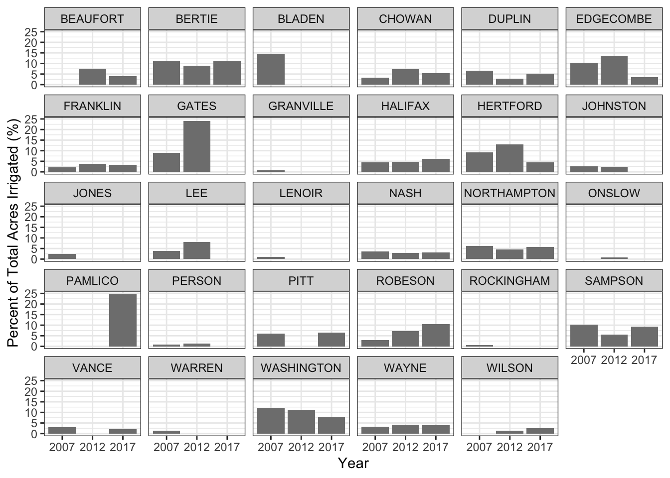
Let’s plot just the counties that have all three years of data available.
# select counties that have all three years
nc_irrigated_mult_years <- nc_irrigated %>%
  group_by(county_name) %>%
  filter(n()>2)

# plot
ggplot(nc_irrigated_mult_years) +
  geom_col(aes(x = factor(year), y = percent_irrigated), fill = "grey50") +
  facet_wrap(~county_name) +
  xlab("Year") +
  ylab("Percent of Total Acres Irrigated (%)") +
  theme_bw()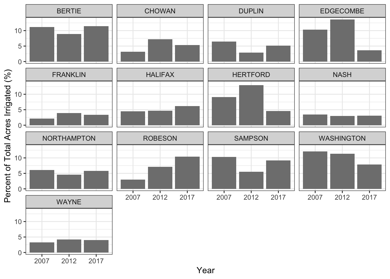
Looking at this figure, it’s hard to see any big patterns in the NASS irrigation data so I summarized the total number of acres irrigated for all 13 counties using summarize().
nc_irrigated_summary <- nc_irrigated_mult_years %>%
  group_by(year) %>%
  summarize(sum_irrigated_ac = sum(irrigated),
            sum_all_production_ac = sum(all_production_practices)) %>%
  mutate(percent_irrigated = (sum_irrigated_ac/sum_all_production_ac) * 100)

nc_irrigated_summary
## # A tibble: 3 x 4
##    year sum_irrigated_ac sum_all_production_ac percent_irrigated
##   <int>            <dbl>                 <dbl>             <dbl>
## 1  2007            46882                700190              6.70
## 2  2012            36687                590884              6.21
## 3  2017            30410                454276              6.69
For this it looks like these 13 counties irrigated about 6.7% of their land in production for 2007 and 2017.
Besides making some bar charts I also mapped the irrigation percentages by county. For this visualization, first, I wanted to keep only 2017 data.
nc_irrigated_2017 <- nc_irrigated %>%
  filter(year == 2017)
Next I used the get_acs() function in the tidycensus package with geometry = TRUE to download the TIGER county boundaries shape (.shp) file for NC. The variable used here (i.e., “B19013_001”) represents median income but you can use any variable you wish. I was interested in the spatial data associated with this and will ignore the tabular (i.e., median income) data.
nc_counties <- get_acs(geography = "county", state = "NC", variables = "B19013_001", year = 2017, geometry = TRUE, survey = "acs5")The second last step is to join nc_irrigated_2017 to the county boundary spatial data.
nc_irrigated_map_2017 <- left_join(nc_counties, nc_irrigated_2017, by = "GEOID")Now I used mapview() to make an interactive plot where counties are colored based on the percentage of irrigated land. You can hover your mouse over the counties to see the actual percentages.
mapviewOptions(vector.palette = colorRampPalette(c("snow", "darkblue", "grey10")))
mapview(nc_irrigated_map_2017, zcol = "percent_irrigated", legend = FALSE)
Some other thoughts that I wanted to mention before signing off:
If you look back at my previous blog post, you’ll notice that the initial tidying of the data was a lot easier when the rnassqs package was available to use.
As always, please feel to reach out if you’ve used the NASS API for other applications or have any other questions/ideas!