Background
This post was originally posted on Jan. 4, 2019 but was revised on May 14, 2020.
Application program interfaces (APIs) help users access (“API request”) and retrieve (“API response”) data from web-based, data servers via programs like R, Python, etc. If you’re interested in more details, several others before me have done a great job writing about API’s and R: this post by C. Waldhauser and this post by T. Clavelle.
I recently learned about a few R packages that help users interface directly with APIs and a few of these are especially interesting for water-minded, data loving people like me. For example the tidycensus package developed by Kyle Walker allows R users to access the US Census API and download data directly into their R environment. It’s awesome. Additionally, I previously wrote about the US Geologic Survey and US Environmental Protection Agency’s dataRetrieval package that interfaces with the National Water Information System API. Some APIs will require you to have an API key (e.g., the US Census) while others don’t (e.g., the National Water Information System). The key is meant to ensure security on your end as well as on the end of the API administrator. In the case of the US Census, they can keep track of your queries and also make sure that you have permission to access certain types of data, etc. You can easily request an US Census API key here and read more about the US Census API here.
But what if you’re working with an API that doesn’t already have an R package associated with it? This is the case for the data associated with the US Department of Agriculture National Agricultural Statistics Service (NASS). I could click through the options on NASS’s Quick Stats page on the web and download the data that way; however, I wanted to use R to access the Quick Stats API directly.
Before jumping into the code, just a brief explainer on the NASS API. The NASS API includes two different types of data:
NASS Agriculture Resource Management Survey (ARMS) - This survey includes data on the “production practices, resource use, and economic well-being of America’s farms and ranches” (NASS ARMS Webiste).
NASS Census of Agriculture - This survey is conducted every 5 years and includes data on the number of US farms and ranches and the people who operate them (as long as more than $1000 was raised from associated agricultural goods). It also includes data on land use, land ownership, production practices, income, and expenses (NASS Census of Agriculture Website).
Goals of This Post
The main goal of this blog post is to:
- Download and plot Agriculture Census data from NASS Quick Stats API using R.
Special thanks to Natalie Nelson of NC State University and Andrew Dau of NASS for some of the R code that I modified for this post.
Set Up
First let’s load the R libraries that we’ll need to run the code in this post.
library(httr)
library(jsonlite)
library(tidycensus)
library(tidyverse)
library(mapview)
The httr and jsonlite packages are necessary for interfacing with the Quick Stats API and reformatting API outputs so they can be used in R.
Let’s use the tidycensus package to get some county boundaries. This will provide some spatial context for our analysis.
The tidyverse and mapview packages will help us wrangle and visualize the API outputs.
Census API Set Up
As I mentioned above, many APIs require that you have a personal API key to access the data stored within them. To run the code in this post you’ll need to make sure you request a Census API key (see instructions below) and a NASS API key (see instructions below). Once you have your API keys, keep them all in one safe spot. I recommend a text file somewhere rememberable on your (password protected) computer.
To request a Census API key, you’ll have to go here and fill in your name and organization. Once you submit the key request, the US Census Bureau will email you a Census API key. This key is unique to the name and email you provided so be sure to keep it in a save place.
If you’ve never installed your Census API key in your R session, you’ll want to install your API key for later use.
CENSUS_API_KEY <- "YOUR API KEY GOES HERE"
census_api_key(CENSUS_API_KEY, install = TRUE)

# The second line of code above will make an entry in your .Renviron file called "CENSUS_API_KEY".
If you’ve already installed your Census API key, you should be good to go, but you can always check to make sure it’s in your R environment using the code below.
# check that it's there
Sys.getenv("CENSUS_API_KEY")
If you want to get tabular and spatial census data using the tidycensus package, you’ll need to run the code below each time you start a new R session. Spatial census data includes, for example, census tract boundaries.
options(tigris_use_cache = TRUE)NASS API Set Up
Be sure to also apply for a NASS API key, which I’ll define in a string called NASS_API_KEY. You can apply for a NASS API key here. As with the Census API key, this is unique to you so be sure to keep it in a safe place.
NASS_API_KEY <- "ADD YOUR NASS API KEY HERE"If you want to save your NASS API key to your R environment, you can use the code below. Setting the NASS API key in your R environment will keep it hidden and accessible only to you. This might be important if you’re planning to pass along your script to someone else…or post it on your blog. ;)
To set the NASS API key your R environment you’ll have to navigate to the (hidden) .Renviron file on your computer. Then you will have to add NASS_API_KEY <- "ADD YOUR NASS API KEY HERE" to that text file. Alternatively, you can also use sys.setenv() as indicated below. See this tutorial and this tutorial. You only need to do this once on your computer.
# add NASS_API_KEY to  your .Renviron file
sys.setenv(NASS_API_KEY <- "ADD YOUR NASS API KEY HERE")
Once you’ve added the NASS API key to your computer’s .Renviron file. You’ll have to run the following code each time you start a new R session. This is because you’ll need to remind R that it has this information available in the .Renviron file.
# load your stored NASS_API_KEY it into your current R session
NASS_API_KEY <- Sys.getenv("NASS_API_KEY")
API Data Query
Now, let’s define the NASS url and path.
In the path you’ll have to specify what type of data you want to query. To specify these you can go to https://quickstats.nass.usda.gov/ to see all your commodity options. I haven’t figured out another way to do this but please contact me if you find an alternative.
For this post I selected the “AG_LAND” commodity, which includes information on the acreage of irrigated farm and ranch lands, because this is the wateR blog after all. Other commodities might include specific crops, etc. I also selected the state of North Carolina because it seems to always be the subject of spatial mapping (e.g., see this post) in R and is also where I live. ;) You can also leave off the last “&state_alpha=NC” part of the string to get data from all states.
# NASS url
nass_url <- "http://quickstats.nass.usda.gov"

# commodity description of interest
my_commodity_desc <- "AG LAND"

# short description of interest (i.e., 'data item' on NASS Quick Stats website)
my_short_desc1 <- "AG LAND, IRRIGATED - ACRES"
my_short_desc2 <- "AG LAND - ACRES"

# query start year
my_year <- "2007"

# state of interest
my_state <- "NC"

# final path string
path_nc_irrig_land <- paste0("api/api_GET/?key=", NASS_API_KEY, "&commodity_desc=", my_commodity_desc, "&short_desc=", my_short_desc1, "&short_desc=", my_short_desc2, "&year__GE=", my_year, "&state_alpha=", my_state)
Let’s query the NASS API.
raw_result_nc_irrig_land <- GET(url = nass_url, path = path_nc_irrig_land)You can check to see if it worked by looking at status_code. To read more about the different status codes and their meaning you can visit https://en.wikipedia.org/wiki/List_of_HTTP_status_codes.
raw_result_nc_irrig_land$status_code
## [1] 200
Great! We want to see status code 200 here. It means our query was received and responded to.
Reformatting API Query Output
If you look at this in your R session, it will come in as a ‘Large response’ or in other words as a JSON object. For simplicity sake, you can think of this as a list of lists (i.e., nested lists). Let’s convert this to a data frame because it’s a little easier to view in R.
We’ll start unpacking the JSON object using rawToChar(). We can check the size and look at the first few characters.
char_raw_nc_irrig_land <- rawToChar(raw_result_nc_irrig_land$content)

# check size of object
nchar(char_raw_nc_irrig_land)
## [1] 3555311

# view first 50 characthers
substr(char_raw_nc_irrig_land, 1, 50)
## [1] "{\"data\":[{\"short_desc\":\"AG LAND, IRRIGATED - ACRES"
This is still a little hard to work with so let’s use fromJSON() and convert the raw character strings to a large list. Due to recent (early 2020) updates to NASS, they now have the data saved in a “data” element of the JSON output.
list_raw_nc_irrig_land <- fromJSON(char_raw_nc_irrig_land)

# keep data element
nc_irrig_land_raw_data <- list_raw_nc_irrig_land$data

# look at the data frame
head(nc_irrig_land_raw_data)
##                   short_desc asd_desc CV (%) source_desc zip_5
## 1 AG LAND, IRRIGATED - ACRES             2.9      CENSUS
## 2 AG LAND, IRRIGATED - ACRES             6.2      CENSUS
## 3 AG LAND, IRRIGATED - ACRES             9.0      CENSUS
## 4 AG LAND, IRRIGATED - ACRES            74.2      CENSUS
## 5 AG LAND, IRRIGATED - ACRES            12.0      CENSUS
## 6 AG LAND, IRRIGATED - ACRES            15.6      CENSUS
##   congr_district_code unit_desc           load_time state_fips_code week_ending
## 1                         ACRES 2012-12-31 00:00:00              37
## 2                         ACRES 2012-12-31 00:00:00              37
## 3                         ACRES 2012-12-31 00:00:00              37
## 4                         ACRES 2012-12-31 00:00:00              37
## 5                         ACRES 2012-12-31 00:00:00              37
## 6                         ACRES 2012-12-31 00:00:00              37
##   county_name agg_level_desc commodity_desc county_code statisticcat_desc
## 1                      STATE        AG LAND                          AREA
## 2                      STATE        AG LAND                          AREA
## 3                      STATE        AG LAND                          AREA
## 4                      STATE        AG LAND                          AREA
## 5                      STATE        AG LAND                          AREA
## 6                      STATE        AG LAND                          AREA
##   region_desc county_ansi  location_desc country_code watershed_code
## 1                         NORTH CAROLINA         9000       00000000
## 2                         NORTH CAROLINA         9000       00000000
## 3                         NORTH CAROLINA         9000       00000000
## 4                         NORTH CAROLINA         9000       00000000
## 5                         NORTH CAROLINA         9000       00000000
## 6                         NORTH CAROLINA         9000       00000000
##                                                             domaincat_desc
## 1                                                 OPERATORS: (1 OPERATORS)
## 2                                         OPERATORS: (2 OR MORE OPERATORS)
## 3               OPERATORS, PRINCIPAL: (PRIMARY OCCUPATION, (EXCL FARMING))
## 4 OPERATORS, PRINCIPAL: (PRIMARY OCCUPATION, (EXCL FARMING), AGE 25 TO 34)
## 5 OPERATORS, PRINCIPAL: (PRIMARY OCCUPATION, (EXCL FARMING), AGE 35 TO 44)
## 6 OPERATORS, PRINCIPAL: (PRIMARY OCCUPATION, (EXCL FARMING), AGE 45 TO 54)
##            domain_desc     state_name state_ansi            group_desc
## 1            OPERATORS NORTH CAROLINA         37 FARMS & LAND & ASSETS
## 2            OPERATORS NORTH CAROLINA         37 FARMS & LAND & ASSETS
## 3 OPERATORS, PRINCIPAL NORTH CAROLINA         37 FARMS & LAND & ASSETS
## 4 OPERATORS, PRINCIPAL NORTH CAROLINA         37 FARMS & LAND & ASSETS
## 5 OPERATORS, PRINCIPAL NORTH CAROLINA         37 FARMS & LAND & ASSETS
## 6 OPERATORS, PRINCIPAL NORTH CAROLINA         37 FARMS & LAND & ASSETS
##    class_desc  sector_desc  Value year begin_code reference_period_desc
## 1 ALL CLASSES DEMOGRAPHICS 76,221 2012         00                  YEAR
## 2 ALL CLASSES DEMOGRAPHICS 98,305 2012         00                  YEAR
## 3 ALL CLASSES DEMOGRAPHICS 21,912 2012         00                  YEAR
## 4 ALL CLASSES DEMOGRAPHICS    669 2012         00                  YEAR
## 5 ALL CLASSES DEMOGRAPHICS  2,131 2012         00                  YEAR
## 6 ALL CLASSES DEMOGRAPHICS  7,379 2012         00                  YEAR
##          util_practice_desc state_alpha prodn_practice_desc freq_desc asd_code
## 1 ALL UTILIZATION PRACTICES          NC           IRRIGATED    ANNUAL
## 2 ALL UTILIZATION PRACTICES          NC           IRRIGATED    ANNUAL
## 3 ALL UTILIZATION PRACTICES          NC           IRRIGATED    ANNUAL
## 4 ALL UTILIZATION PRACTICES          NC           IRRIGATED    ANNUAL
## 5 ALL UTILIZATION PRACTICES          NC           IRRIGATED    ANNUAL
## 6 ALL UTILIZATION PRACTICES          NC           IRRIGATED    ANNUAL
##    country_name watershed_desc end_code
## 1 UNITED STATES                      00
## 2 UNITED STATES                      00
## 3 UNITED STATES                      00
## 4 UNITED STATES                      00
## 5 UNITED STATES                      00
## 6 UNITED STATES                      00
This looks ok but there are still some things that would be nice to clean up. As mentioned above, I wanted to focus on the acres of irrigated lands in NC. For simplicity, I’ll only look at farms/ranches with 2,000 ac or more under operation. Let’s step through each line in the piped (i.e., %>%) code below. See the in-line comments for the details.
nc_irrigated <- nc_irrig_land_raw_data %>%

  # filter to select county level irrigation data where farms/ranches with 2,000+ ac operation and irrigation status to get total acres of ag land in county
  filter(agg_level_desc == "COUNTY") %>%
  filter(unit_desc == "ACRES") %>%
  filter(domaincat_desc == "AREA OPERATED: (2,000 OR MORE ACRES)" | domaincat_desc == "IRRIGATION STATUS: (ANY ON OPERATION)") %>%

  # trim white space from ends (note: 'Value' is a character here, not a number)
  mutate(value_trim = str_trim(Value)) %>%

  # select only the columns we'll need
  select(state_name, state_alpha, state_ansi, county_code, county_name, asd_desc,
         agg_level_desc, year, prodn_practice_desc_char = prodn_practice_desc, domaincat_desc,
         short_desc, value_ac_per_yr_char=value_trim, unit_desc) %>%

  # filter out entries with codes '(D)' and '(Z)'
  filter(value_ac_per_yr_char != "(D)" & value_ac_per_yr_char != "(Z)") %>%

  # remove commas from number values and convert to R numeric class
  mutate(value_ac_per_yr = as.numeric(str_remove(value_ac_per_yr_char, ","))) %>%

  # change blanks to underscores in prodn_practice_desc_char for latter processing
  mutate(prodn_practice_desc = str_replace_all(str_to_lower(prodn_practice_desc_char),
                                               "[ ]", "_")) %>%

  # remove unnecessary columns
  select(-value_ac_per_yr_char, -prodn_practice_desc_char) %>%
  #arrange(county_code, year)

  # we have 2007, 2012, and 2017 data and we want irrigated land acreage and total land acreage
  # (to calculate a percentage of irrigated land) so we use n()>1 to filter out counties
  # that have both types of acreage for each year
  group_by(county_code, year) %>%
  filter(n()>1) %>%

  # drop columns we don't need
  select(-domaincat_desc, -short_desc) %>%

  # pivot wide irrigated and total lands operated data and calculate percent irrigated
  pivot_wider(names_from = prodn_practice_desc, values_from = value_ac_per_yr) %>%
  mutate(percent_irrigated = round(irrigated/all_production_practices*100, 1)) %>%

  # make a column with the county name and year (we'll need this for plotting)
  mutate(county_year = paste0(str_to_lower(county_name), "_", year)) %>%

  # make GEOID column to match up with county level spatial data (we'll need this for mapping)
  mutate(GEOID = paste0(state_ansi, county_code)) %>%
  ungroup()
Let’s look at the first few rows of the final reformatted NASS data showing the amount of irrigated acres in NC for 2007, 2012, and 2017.
head(nc_irrigated)
## # A tibble: 6 x 14
##   state_name state_alpha state_ansi county_code county_name asd_desc
##   <chr>      <chr>       <chr>      <chr>       <chr>       <chr>
## 1 NORTH CAR… NC          37         069         FRANKLIN    NORTHER…
## 2 NORTH CAR… NC          37         069         FRANKLIN    NORTHER…
## 3 NORTH CAR… NC          37         069         FRANKLIN    NORTHER…
## 4 NORTH CAR… NC          37         077         GRANVILLE   NORTHER…
## 5 NORTH CAR… NC          37         145         PERSON      NORTHER…
## 6 NORTH CAR… NC          37         145         PERSON      NORTHER…
## # … with 8 more variables: agg_level_desc <chr>, year <int>, unit_desc <chr>,
## #   all_production_practices <dbl>, irrigated <dbl>, percent_irrigated <dbl>,
## #   county_year <chr>, GEOID <chr>
Plotting NASS Data
Now that we have this nicely formatted data, let’s make some figures!
I started by making bar charts comparing the percentage of irrigated land in NC counties where data with available data for 2007, 2012, and 2017.
ggplot(nc_irrigated) +
  geom_col(aes(x = factor(year), y = percent_irrigated), fill = "grey50") +
  facet_wrap(~county_name) +
  xlab("Year") +
  ylab("Percent of Total Acres Irrigated (%)") +
  theme_bw()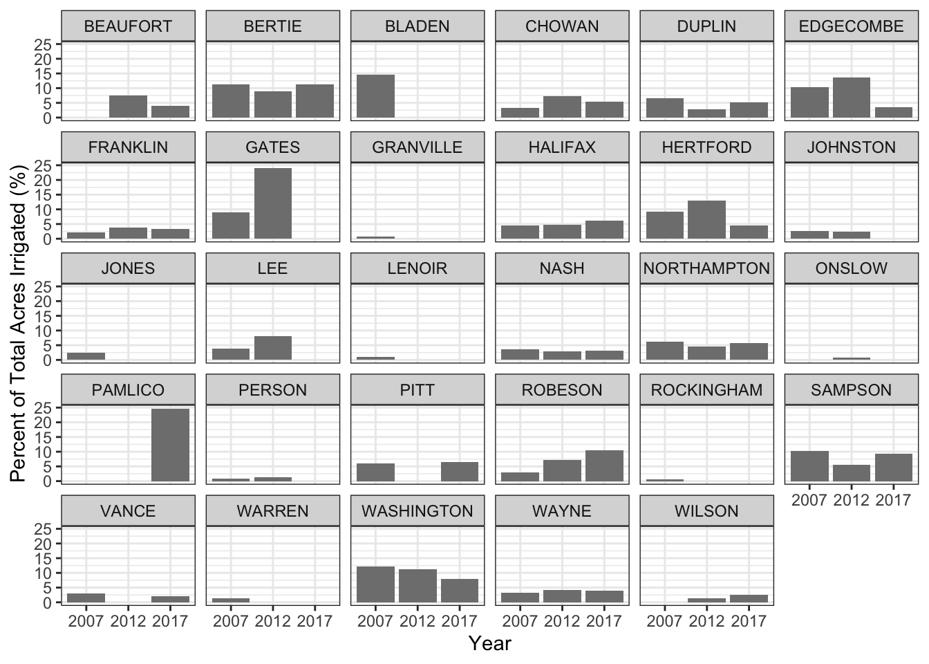
Let’s plot just the counties that have all three years of data available.
# select counties that have all three years
nc_irrigated_mult_years <- nc_irrigated %>%
  group_by(county_name) %>%
  filter(n()>2)

# plot
ggplot(nc_irrigated_mult_years) +
  geom_col(aes(x = factor(year), y = percent_irrigated), fill = "grey50") +
  facet_wrap(~county_name) +
  xlab("Year") +
  ylab("Percent of Total Acres Irrigated (%)") +
  theme_bw()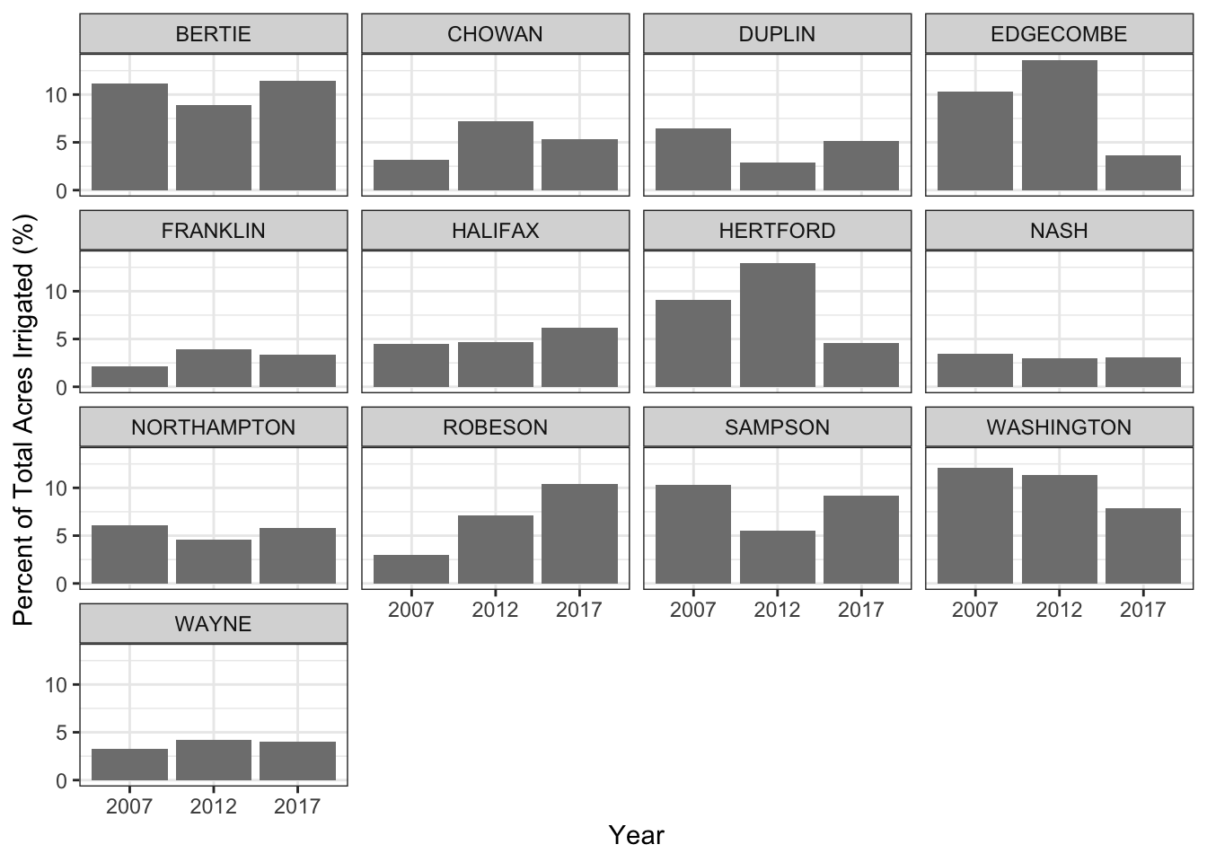
Looking at this figure, it’s hard to see any big patterns in the NASS irrigation data so I summarized the total number of acres irrigated for all 13 counties using summarize().
nc_irrigated_summary <- nc_irrigated_mult_years %>%
  group_by(year) %>%
  summarize(sum_irrigated_ac = sum(irrigated),
            sum_all_production_ac = sum(all_production_practices)) %>%
  mutate(percent_irrigated = (sum_irrigated_ac/sum_all_production_ac) * 100)

nc_irrigated_summary
## # A tibble: 3 x 4
##    year sum_irrigated_ac sum_all_production_ac percent_irrigated
##   <int>            <dbl>                 <dbl>             <dbl>
## 1  2007            46882                700190              6.70
## 2  2012            36687                590884              6.21
## 3  2017            30410                454276              6.69
For this it looks like these 13 counties irrigated about 6.7% of their land in production for 2007 and 2017.
Besides making some bar charts I also mapped the irrigation percentages by county. For this visualization, first, I wanted to keep only 2017 data.
nc_irrigated_2017 <- nc_irrigated %>%
  filter(year == 2017)
Next I used the get_acs() function in the tidycensus package with geometry = TRUE to download the TIGER county boundaries shape (.shp) file for NC. The variable used here (i.e., “B19013_001”) represents median income but you can use any variable you wish. I was interested in the spatial data associated with this and will ignore the tabular (i.e., median income) data.
nc_counties <- get_acs(geography = "county", state = "NC", variables = "B19013_001", year = 2017, geometry = TRUE, survey = "acs5")The second last step is to join nc_irrigated_2017 to the county boundary spatial data.
nc_irrigated_map_2017 <- left_join(nc_counties, nc_irrigated_2017, by = "GEOID")Now I used mapview() to make an interactive plot where counties are colored based on the percentage of irrigated land. You can hover your mouse over the counties to see the actual percentages.
mapviewOptions(vector.palette = colorRampPalette(c("snow", "darkblue", "grey10")))
mapview(nc_irrigated_map_2017, zcol = "percent_irrigated", legend = FALSE)
Some other thoughts that I wanted to mention before signing off:
Querying the NASS API was fairly straightforward, and despite needing to do some considerable data wrangling with the output, the
tidyversepackages (i.e.,dplyrandtidyr) helped a lot. I should note that I spent some time figuring out what the query outputs would look like for different commodities and what aspects of the query outputs I needed.It was interesting to see that a higher percentage of acres were irrigated in NC in 2007 compared to 2012. I can’t say what caused these differences based on these data alone, but it would be interesting to look into whether this finding was linked to the 2007 drought. According to other scientists who lived and researched water resources at the time, the 2007 drought affected millions of people in NC. A longer time series of irrigated land might help with this as would overlapping these county level results with drought reports and crop losses.
I can think of a number of other commodities that might be interesting to look at in the NASS Quick Stats data set. I’m assuming that some commonly farmed commodities (i.e., corn) might have more years and locations available. If you’ve used the NASS API for other applications or have any other questions/ideas please let me know!
Updates Since Posting
June 2020: NASS updated the format of their database so the data is saved in a data element of the JSON list. Thus, this post no longer requires the purrr package to run.
June 2019: Looks like NASS has officially published a usdarnass package to CRAN! You can read the package documentation here. Looks like there are some nice look-up tables which might be very helpful.
January 2019: Since first posting this, Julian Reyes suggested using Nicholas Potter’s package called rnassqs to help automate the NASS API portion of this post. You can read more about the rnassqs package here. Note to self that I need to check it out!