Background
I recently participated in Thomas Mock’s Tidy Tuesday R challenge with other members of the NC State University R Learning Group. It was a lot of fun and after participating, I felt motivated to share what I’ve been doing to tidy up my own data sets.
Specifically, I’ve been working with collaborator, Kelly Suttles, to tidy up model outputs from the Soil and Water Assessment Tool (SWAT). SWAT is a hydrologic model used to predict daily and monthly streamflow and water quality at the watershed-scale. It’s pretty widely used and there are even some existing R packages to help researchers calibrate SWAT from the R command line. These include the ecohydRology package and the SWATmodel package. Check them out if you work with SWAT and use R.
I’m sure there are a lot of researchers out there who have developed their own ways of tidying up SWAT outputs but I thought it would be helpful to share some of the functions I’ve recently created to help Kelly migrate her SWAT output analysis from Excel to R.
Goals of This Post
The goals of this blog post are to:
- Discuss how to tidy up SWAT daily and monthly outputs.
- Create functions to make tidying up SWAT outputs easier.
- Share reproducible data analysis workflows.
Special thanks to Kelly Suttles for generating and sharing these SWAT outputs with me.
If you’re interested in reading more about what Kelly and I have been doing with SWAT outputs, you can read Kelly’s recently paper published in Science of the Total Environment here. I’m currently working on a second paper that relies on Kelly’s SWAT model outputs and I’ll update this post once that’s published.
Please feel free to use the functions below for your own SWAT output tidying and analysis! Please contact me on Twitter or any other method here if you find any mistakes, have suggestions, or know of any other SWAT data analysis resources for R.
First let’s load the R libraries that we’ll need to run the code in this post.
library(tidyverse)
library(lubridate)
Daily Data
Next let’s load the daily SWAT outputs first (we’ll work on monthly outputs later). These are generated by SWAT and can be found in the SWAT project Scenarios > Default > TxtInOut directory. In this post, I’ll just be working with the output.rch files, which represent the main channel outputs for each subbasin within the larger, SWAT delineated watershed. You can read more about the different SWAT output files here. In this particular example, I’ll be working with SWAT outputs from the Yadkin-Pee Dee River Watershed (YPD) in North Carolina, USA. The YPD has 28 subbasins as delineated by SWAT.
# define data folder paths
daily_data_path <- paste0(here::here(), "/static/data/2018-10-16-tidy-swat/daily/output.rch")

# load daily data
output_daily_rch_raw <- read_csv(daily_data_path)

head(output_daily_rch_raw)
## # A tibble: 6 x 1
##   `1`
##   <chr>
## 1 SWAT May 20 2015    VER 2015/Rev 637                                         …
## 2 General Input/Output section (file.cio):
## 3 9/30/2016 12:00:00 AM ARCGIS-SWAT interface AV
## 4 RCH      GIS  MO DA   YR     AREAkm2  FLOW_INcms FLOW_OUTcms     EVAPcms    T…
## 5 REACH    1        0   1  1 1982   0.8080E+03  0.1230E+02  0.1260E+02  0.1868E…
## 6 REACH    2        0   1  1 1982   0.3187E+04  0.1486E+03  0.1538E+03  0.6552E…
Using the basic read_csv() and without doing any formatting, we notice a few things:
- These data are being read in as one big column
- There are several lines of text describing the
output.rchfile before the data begins - Several of the column names have characters that R might not like (e.g., / and a space)
Let’s skip the first 9 columns and set the header argument to false. We’ll manually add the header names later, and when we do, we can reformat the column names using tidy principles (i.e., no / and no spaces). We can also use read_table2() instead of read_csv() to deal with the unequal spacing between columns in the text file. More specifically, if you open the output.rch file in a text editor, you’ll notice that the month column doesn’t always have the same number of spaces before the month number. If you just use read_table() you’ll loose the first digit of months 10, 11, and 12, which is not good for downstream data analysis. (I know from personal experience.)
output_daily_rch_raw <- read_table2(daily_data_path, skip = 9, col_names = FALSE)

head(output_daily_rch_raw, n = 5)
## # A tibble: 5 x 53
##   X1       X2    X3    X4    X5    X6    X7    X8    X9     X10   X11    X12
##   <chr> <dbl> <dbl> <dbl> <dbl> <dbl> <dbl> <dbl> <dbl>   <dbl> <dbl>  <dbl>
## 1 REACH     1     0     1     1  1982  808   12.3  12.6 1.87e-2     0 3.49e1
## 2 REACH     2     0     1     1  1982 3187  149.  154.  6.55e-2     0 1.76e3
## 3 REACH     3     0     1     1  1982 2238  138.  141.  4.33e-2     0 2.01e3
## 4 REACH     4     0     1     1  1982 4365  170.  170.  5.45e-2     0 1.89e3
## 5 REACH     5     0     1     1  1982  625. 107.  107.  1.50e-5     0 2.10e5
## # … with 41 more variables: X13 <dbl>, X14 <dbl>, X15 <dbl>, X16 <dbl>,
## #   X17 <dbl>, X18 <dbl>, X19 <dbl>, X20 <dbl>, X21 <dbl>, X22 <dbl>,
## #   X23 <dbl>, X24 <dbl>, X25 <dbl>, X26 <dbl>, X27 <dbl>, X28 <dbl>,
## #   X29 <dbl>, X30 <dbl>, X31 <dbl>, X32 <dbl>, X33 <dbl>, X34 <dbl>,
## #   X35 <dbl>, X36 <dbl>, X37 <dbl>, X38 <dbl>, X39 <dbl>, X40 <dbl>,
## #   X41 <dbl>, X42 <dbl>, X43 <dbl>, X44 <dbl>, X45 <dbl>, X46 <dbl>,
## #   X47 <dbl>, X48 <dbl>, X49 <dbl>, X50 <dbl>, X51 <dbl>, X52 <dbl>, X53 <dbl>
That looks a lot better but we still need to add header names. You can find additional descriptions on these column names in the SWAT output.rch documentation
# create a new dataframe to save final output
output_daily_rch <- output_daily_rch_raw

# column names list
daily_rch_col_names <- c("FILE","RCH","GIS","MO","DA","YR","AREAkm2","FLOW_INcms","FLOW_OUTcms","EVAPcms","TLOSScms","SED_INtons","SED_OUTtons","SEDCONCmg_kg","ORGN_INkg","ORGN_OUTkg","ORGP_INkg","ORGP_OUTkg","NO3_INkg","NO3_OUTkg","NH4_INkg","NH4_OUTkg","NO2_INkg","NO2_OUTkg","MINP_INkg","MINP_OUTkg","CHLA_INkg","CHLA_OUTkg","CBOD_INkg","CBOD_OU/.Tkg","DISOX_INkg","DISOX_OUTkg","SOLPST_INmg","SOLPST_OUTmg","SORPST_INmg","SORPST_OUTmg","REACTPSTmg","VOLPSTmg","SETTLPSTmg","RESUSP_PSTmg","DIFFUSEPSTmg","REACBEDPSTmg","BURYPSTmg","BED_PSTmg","BACTP_OUTct","BACTLP_OUTct","CMETAL_1kg","CMETAL_2kg","CMETAL_3kg","TOTNkg","TOTPkg","NO3_mg_l","WTMPdegc")

# reassign column names
colnames(output_daily_rch) <- daily_rch_col_names

head(output_daily_rch, n = 5)
## # A tibble: 5 x 53
##   FILE    RCH   GIS    MO    DA    YR AREAkm2 FLOW_INcms FLOW_OUTcms EVAPcms
##   <chr> <dbl> <dbl> <dbl> <dbl> <dbl>   <dbl>      <dbl>       <dbl>   <dbl>
## 1 REACH     1     0     1     1  1982    808        12.3        12.6 1.87e-2
## 2 REACH     2     0     1     1  1982   3187       149.        154.  6.55e-2
## 3 REACH     3     0     1     1  1982   2238       138.        141.  4.33e-2
## 4 REACH     4     0     1     1  1982   4365       170.        170.  5.45e-2
## 5 REACH     5     0     1     1  1982    625.      107.        107.  1.50e-5
## # … with 43 more variables: TLOSScms <dbl>, SED_INtons <dbl>,
## #   SED_OUTtons <dbl>, SEDCONCmg_kg <dbl>, ORGN_INkg <dbl>, ORGN_OUTkg <dbl>,
## #   ORGP_INkg <dbl>, ORGP_OUTkg <dbl>, NO3_INkg <dbl>, NO3_OUTkg <dbl>,
## #   NH4_INkg <dbl>, NH4_OUTkg <dbl>, NO2_INkg <dbl>, NO2_OUTkg <dbl>,
## #   MINP_INkg <dbl>, MINP_OUTkg <dbl>, CHLA_INkg <dbl>, CHLA_OUTkg <dbl>,
## #   CBOD_INkg <dbl>, `CBOD_OU/.Tkg` <dbl>, DISOX_INkg <dbl>, DISOX_OUTkg <dbl>,
## #   SOLPST_INmg <dbl>, SOLPST_OUTmg <dbl>, SORPST_INmg <dbl>,
## #   SORPST_OUTmg <dbl>, REACTPSTmg <dbl>, VOLPSTmg <dbl>, SETTLPSTmg <dbl>,
## #   RESUSP_PSTmg <dbl>, DIFFUSEPSTmg <dbl>, REACBEDPSTmg <dbl>,
## #   BURYPSTmg <dbl>, BED_PSTmg <dbl>, BACTP_OUTct <dbl>, BACTLP_OUTct <dbl>,
## #   CMETAL_1kg <dbl>, CMETAL_2kg <dbl>, CMETAL_3kg <dbl>, TOTNkg <dbl>,
## #   TOTPkg <dbl>, NO3_mg_l <dbl>, WTMPdegc <dbl>
That’s so tidy! We can summarize all those steps into one function that we’ll call tidy_daily_rch_file() that takes the raw input that we’ve read in (using read_table2("output.rch", col_names=FALSE, skip=9)) and outputs a formatted daily SWAT output table.
tidy_daily_rch_file <- function(daily_rch_raw_data) {
  # import daily_rch_raw_data into R session using:
  # daily_rch_raw_data <- read_table2("output.rch", col_names=FALSE, skip=9)

  # column names
  daily_rch_col_names <- c("FILE","RCH","GIS","MO","DA","YR","AREAkm2","FLOW_INcms","FLOW_OUTcms","EVAPcms","TLOSScms","SED_INtons","SED_OUTtons","SEDCONCmg_kg","ORGN_INkg","ORGN_OUTkg","ORGP_INkg","ORGP_OUTkg","NO3_INkg","NO3_OUTkg","NH4_INkg","NH4_OUTkg","NO2_INkg","NO2_OUTkg","MINP_INkg","MINP_OUTkg","CHLA_INkg","CHLA_OUTkg","CBOD_INkg","CBOD_OU/.Tkg","DISOX_INkg","DISOX_OUTkg","SOLPST_INmg","SOLPST_OUTmg","SORPST_INmg","SORPST_OUTmg","REACTPSTmg","VOLPSTmg","SETTLPSTmg","RESUSP_PSTmg","DIFFUSEPSTmg","REACBEDPSTmg","BURYPSTmg","BED_PSTmg","BACTP_OUTct","BACTLP_OUTct","CMETAL_1kg","CMETAL_2kg","CMETAL_3kg","TOTNkg","TOTPkg","NO3_mg_l","WTMPdegc")

  # reassign column names
  colnames(daily_rch_raw_data) <- daily_rch_col_names

  # return output
  return(daily_rch_raw_data)
}
So now it will just take two lines of code to read in our daily SWAT output.rch file and tidy it up!
output_daily_rch_raw_test <- read_table2(daily_data_path, skip = 9, col_names = FALSE)

output_daily_rch_test <- tidy_daily_rch_file(output_daily_rch_raw_test)

head(output_daily_rch_test, n = 5)
## # A tibble: 5 x 53
##   FILE    RCH   GIS    MO    DA    YR AREAkm2 FLOW_INcms FLOW_OUTcms EVAPcms
##   <chr> <dbl> <dbl> <dbl> <dbl> <dbl>   <dbl>      <dbl>       <dbl>   <dbl>
## 1 REACH     1     0     1     1  1982    808        12.3        12.6 1.87e-2
## 2 REACH     2     0     1     1  1982   3187       149.        154.  6.55e-2
## 3 REACH     3     0     1     1  1982   2238       138.        141.  4.33e-2
## 4 REACH     4     0     1     1  1982   4365       170.        170.  5.45e-2
## 5 REACH     5     0     1     1  1982    625.      107.        107.  1.50e-5
## # … with 43 more variables: TLOSScms <dbl>, SED_INtons <dbl>,
## #   SED_OUTtons <dbl>, SEDCONCmg_kg <dbl>, ORGN_INkg <dbl>, ORGN_OUTkg <dbl>,
## #   ORGP_INkg <dbl>, ORGP_OUTkg <dbl>, NO3_INkg <dbl>, NO3_OUTkg <dbl>,
## #   NH4_INkg <dbl>, NH4_OUTkg <dbl>, NO2_INkg <dbl>, NO2_OUTkg <dbl>,
## #   MINP_INkg <dbl>, MINP_OUTkg <dbl>, CHLA_INkg <dbl>, CHLA_OUTkg <dbl>,
## #   CBOD_INkg <dbl>, `CBOD_OU/.Tkg` <dbl>, DISOX_INkg <dbl>, DISOX_OUTkg <dbl>,
## #   SOLPST_INmg <dbl>, SOLPST_OUTmg <dbl>, SORPST_INmg <dbl>,
## #   SORPST_OUTmg <dbl>, REACTPSTmg <dbl>, VOLPSTmg <dbl>, SETTLPSTmg <dbl>,
## #   RESUSP_PSTmg <dbl>, DIFFUSEPSTmg <dbl>, REACBEDPSTmg <dbl>,
## #   BURYPSTmg <dbl>, BED_PSTmg <dbl>, BACTP_OUTct <dbl>, BACTLP_OUTct <dbl>,
## #   CMETAL_1kg <dbl>, CMETAL_2kg <dbl>, CMETAL_3kg <dbl>, TOTNkg <dbl>,
## #   TOTPkg <dbl>, NO3_mg_l <dbl>, WTMPdegc <dbl>
Now can use output_daily_rch_test for some downstream data analysis. Let’s first plot the range in monthly discharge (as predicted by SWAT) just at the outlet (i.e., subbasin number 28) versus the simulation year.
# select outlet data
outlet_daily_data <- output_daily_rch_test %>%
  filter(RCH == 28)

# plot
ggplot(data = outlet_daily_data, mapping = aes(x = as.factor(YR), y = FLOW_OUTcms)) +
  geom_boxplot() +
  geom_jitter(alpha = 0.1, width = 0.1) +
  xlab("Year") +
  ylab("Daily Discharge (cms)")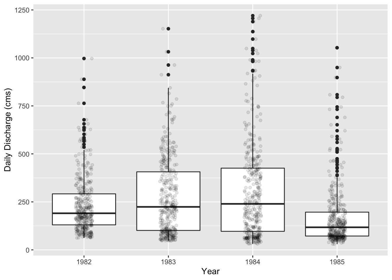
Next, let’s plot the hydrograph of discharge at the the outlet (i.e., subbasin number 28) for 1982.
# select outlet data for 1982
outlet_daily_1982_data <- output_daily_rch_test %>%
  filter(RCH == 28) %>%
  filter(YR == 1982) %>%
  mutate(date = as.Date(paste0(YR,"-",MO,"-",DA)))

ggplot(data = outlet_daily_1982_data, mapping = aes(x = date, y = FLOW_OUTcms)) +
  geom_line(color = "blue") +
  xlab("Date") +
  ylab("Daily Discharge (cms)")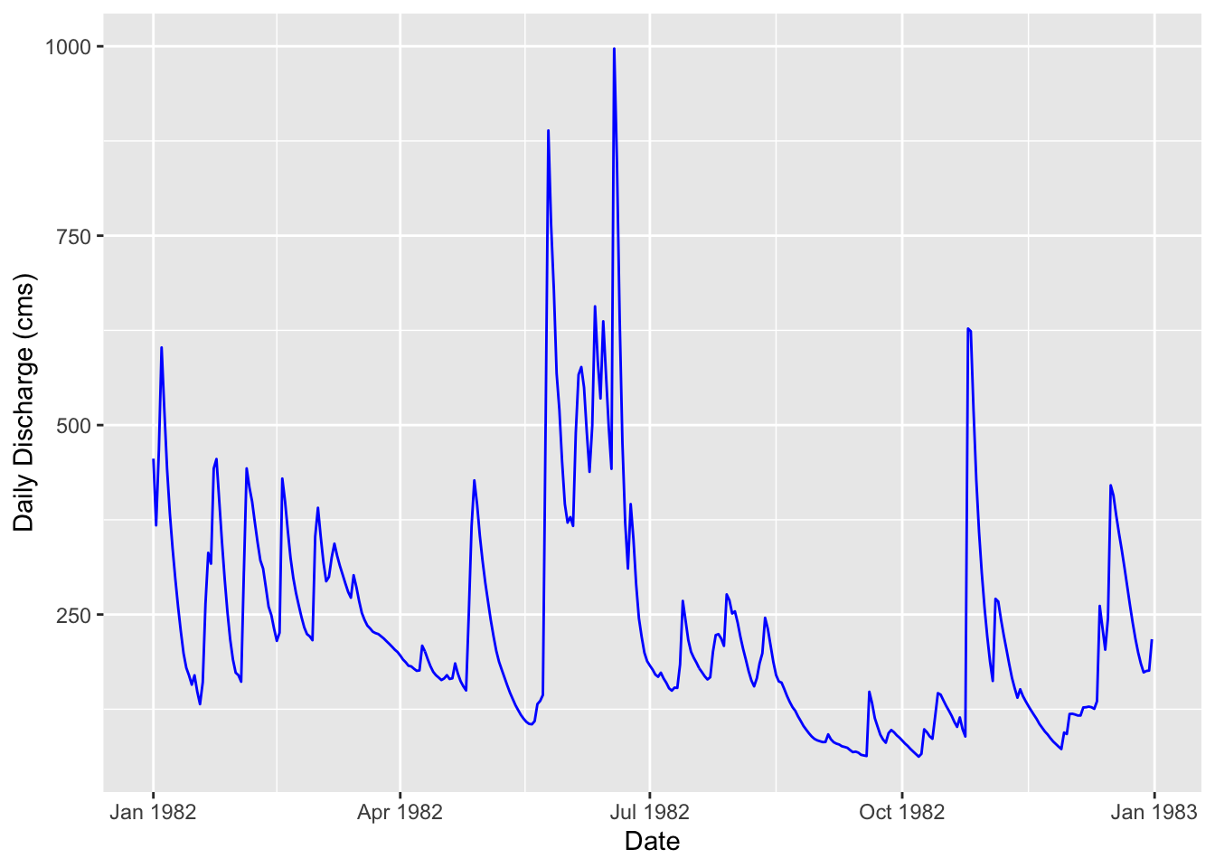
Monthly Data
You can also run SWAT at a monthly time-step. This might happen if you are trying to predict sediment or nutrient loads when you only have these measurements at the monthly time-step. The SWAT output.rch file is slightly different if you use the monthly time-step. More on this later.
# define data folder paths
monthly_data_path <- paste0(here::here(), "/static/data/2018-10-16-tidy-swat/monthly/output.rch")

# load daily data
output_monthly_rch_raw <- read_csv(monthly_data_path)

head(output_monthly_rch_raw)
## # A tibble: 6 x 1
##   `1`
##   <chr>
## 1 SWAT May 20 2015    VER 2015/Rev 637                                         …
## 2 General Input/Output section (file.cio):
## 3 9/1/2017 12:00:00 AM ARCGIS-SWAT interface AV
## 4 RCH      GIS   MON     AREAkm2  FLOW_INcms FLOW_OUTcms     EVAPcms    TLOSScm…
## 5 REACH    1        0     1  0.8080E+03  0.3818E+01  0.3911E+01  0.1456E-01  0.…
## 6 REACH    2        0     1  0.3187E+04  0.1997E+02  0.2023E+02  0.5534E-01  0.…
Using the basic read_csv() and without doing any formatting, we notice a few things:
- These data are being read in as one big column (Like the daily data!)
- There are several lines of text describing the
output.rchfile before the data begins (Like the daily data!) - Several of the column names have characters that R might not like (e.g., / and a space) (Like the daily data!)
- The year of the simulation is included in the MO (i.e., month) and represents a summary of the data for that year (This is new to the month file.)
- There is no YR column (This is new to the month file.)
If we use the same formatting we used before with the daily data and skip down to the 336 row, the fourth point above becomes more clear.
# read in monthly data
output_monthly_rch_raw <- read_table2(monthly_data_path, skip = 9, col_names = FALSE)

# column names
montly_rch_col_names=c("FILE","RCH","GIS","MO","AREAkm2","FLOW_INcms","FLOW_OUTcms","EVAPcms","TLOSScms","SED_INtons","SED_OUTtons","SEDCONCmg_kg","ORGN_INkg","ORGN_OUTkg","ORGP_INkg","ORGP_OUTkg","NO3_INkg","NO3_OUTkg","NH4_INkg","NH4_OUTkg","NO2_INkg","NO2_OUTkg","MINP_INkg","MINP_OUTkg","CHLA_INkg","CHLA_OUTkg","CBOD_INkg","CBOD_OUTkg","DISOX_INkg","DISOX_OUTkg","SOLPST_INmg","SOLPST_OUTmg","SORPST_INmg","SORPST_OUTmg","REACTPSTmg","VOLPSTmg","SETTLPSTmg","RESUSP_PSTmg","DIFFUSEPSTmg","REACBEDPSTmg","BURYPSTmg","BED_PSTmg","BACTP_OUTct","BACTLP_OUTct","CMETALnumkg","CMETALnum2kg","CMETALnum3kg","TOTNkg","TOTPkg","NO3ConcMg_l","WTMPdegc")

# reassign column names
colnames(output_monthly_rch_raw) = montly_rch_col_names

output_monthly_rch_raw[336:338,]
## # A tibble: 3 x 51
##   FILE    RCH   GIS    MO AREAkm2 FLOW_INcms FLOW_OUTcms EVAPcms TLOSScms
##   <chr> <dbl> <dbl> <dbl>   <dbl>      <dbl>       <dbl>   <dbl>    <dbl>
## 1 REACH    28     0    12   17780     137.        137.    0.0587     5.66
## 2 REACH     1     0  1982     808       8.47        8.39  0.0658     3.51
## 3 REACH     2     0  1982    3187      42.0        41.7   0.231     12.3
## # … with 42 more variables: SED_INtons <dbl>, SED_OUTtons <dbl>,
## #   SEDCONCmg_kg <dbl>, ORGN_INkg <dbl>, ORGN_OUTkg <dbl>, ORGP_INkg <dbl>,
## #   ORGP_OUTkg <dbl>, NO3_INkg <dbl>, NO3_OUTkg <dbl>, NH4_INkg <dbl>,
## #   NH4_OUTkg <dbl>, NO2_INkg <dbl>, NO2_OUTkg <dbl>, MINP_INkg <dbl>,
## #   MINP_OUTkg <dbl>, CHLA_INkg <dbl>, CHLA_OUTkg <dbl>, CBOD_INkg <dbl>,
## #   CBOD_OUTkg <dbl>, DISOX_INkg <dbl>, DISOX_OUTkg <dbl>, SOLPST_INmg <dbl>,
## #   SOLPST_OUTmg <dbl>, SORPST_INmg <dbl>, SORPST_OUTmg <dbl>,
## #   REACTPSTmg <dbl>, VOLPSTmg <dbl>, SETTLPSTmg <dbl>, RESUSP_PSTmg <dbl>,
## #   DIFFUSEPSTmg <dbl>, REACBEDPSTmg <dbl>, BURYPSTmg <dbl>, BED_PSTmg <dbl>,
## #   BACTP_OUTct <dbl>, BACTLP_OUTct <dbl>, CMETALnumkg <dbl>,
## #   CMETALnum2kg <dbl>, CMETALnum3kg <dbl>, TOTNkg <dbl>, TOTPkg <dbl>,
## #   NO3ConcMg_l <dbl>, WTMPdegc <dbl>
We see that the month column goes from 12 to 1982; 1982 is the first year of the simulation.
Overall, the monthly SWAT output in combining two types of data (i.e., month number and year number) in one column. Likewise, the data associated with the corresponding rows of these yearly summary columns is lumped together with the monthly SWAT outputs. This is definitely not tidy; tidy data consists of unique variables in each column and unique observations in each row. The easiest way tidy this up is to identify and delete the yearly summary rows. If you want, you can save them for later QA/QC. That is, you can compare the yearly average summaries interspersed within the monthly SWAT output to yearly averages that you manually calculate from the monthly SWAT outputs. In this post, we’ll delete the yearly summary rows.
We’ll keep track of the simulation years, take out the summary rows, and add a column called YR that we’ll fill in the next step.
# record the simulation years for later
simulation_years <- unique(output_monthly_rch_raw$MO)[unique(output_monthly_rch_raw$MO) > 12]
num_years <- length(simulation_years)

# remove summary rows but make YR column to hold these data
output_monthly_rch <- output_monthly_rch_raw %>%
  mutate(notes = ifelse(MO > 12, "summary", "not_summary")) %>% # note whether summary or not
  mutate(YR = as.numeric("NA")) %>% # make an empty column to fill later
  filter(notes == "not_summary") %>% # remove annual summary for each subbasin
  select(-notes) %>% # remove it to keep it tidy
  select(FILE:MO, YR, AREAkm2:WTMPdegc) # rearrange columns

dim(output_monthly_rch_raw)
## [1] 1456   51
dim(output_monthly_rch)
## [1] 1344   52
We see output_monthly_rch_raw had 1456 rows and the output_monthly_rch now has 1344. That’s 112 less rows, which checks out because 4 years times 28 subbasins is 112. That is, there was one summary row for each subbasin for each year that we just deleted.
Now let’s loop through the data and fill in the year column.
# define some parameters we'll need
num_subs <- max(unique(output_monthly_rch$RCH))
num_months <- 12
num_per_month <- num_subs * num_months

# for loop
str=1
end=num_per_month
for (i in 1:length(simulation_years)) {
  output_monthly_rch$YR[str:end] = rep(simulation_years[i], num_per_month)
  str=end+1
  end=str+num_per_month-1
}

head(output_monthly_rch, n = 5)
## # A tibble: 5 x 52
##   FILE    RCH   GIS    MO    YR AREAkm2 FLOW_INcms FLOW_OUTcms EVAPcms TLOSScms
##   <chr> <dbl> <dbl> <dbl> <dbl>   <dbl>      <dbl>       <dbl>   <dbl>    <dbl>
## 1 REACH     1     0     1  1982    808        3.82        3.91 1.46e-2  3.24
## 2 REACH     2     0     1  1982   3187       20.0        20.2  5.53e-2 11.8
## 3 REACH     3     0     1  1982   2238       15.5        15.9  4.35e-2  8.00
## 4 REACH     4     0     1  1982   4365       25.5        25.4  8.00e-2 10.5
## 5 REACH     5     0     1  1982    625.       8.99        8.99 3.74e-5  0.00429
## # … with 42 more variables: SED_INtons <dbl>, SED_OUTtons <dbl>,
## #   SEDCONCmg_kg <dbl>, ORGN_INkg <dbl>, ORGN_OUTkg <dbl>, ORGP_INkg <dbl>,
## #   ORGP_OUTkg <dbl>, NO3_INkg <dbl>, NO3_OUTkg <dbl>, NH4_INkg <dbl>,
## #   NH4_OUTkg <dbl>, NO2_INkg <dbl>, NO2_OUTkg <dbl>, MINP_INkg <dbl>,
## #   MINP_OUTkg <dbl>, CHLA_INkg <dbl>, CHLA_OUTkg <dbl>, CBOD_INkg <dbl>,
## #   CBOD_OUTkg <dbl>, DISOX_INkg <dbl>, DISOX_OUTkg <dbl>, SOLPST_INmg <dbl>,
## #   SOLPST_OUTmg <dbl>, SORPST_INmg <dbl>, SORPST_OUTmg <dbl>,
## #   REACTPSTmg <dbl>, VOLPSTmg <dbl>, SETTLPSTmg <dbl>, RESUSP_PSTmg <dbl>,
## #   DIFFUSEPSTmg <dbl>, REACBEDPSTmg <dbl>, BURYPSTmg <dbl>, BED_PSTmg <dbl>,
## #   BACTP_OUTct <dbl>, BACTLP_OUTct <dbl>, CMETALnumkg <dbl>,
## #   CMETALnum2kg <dbl>, CMETALnum3kg <dbl>, TOTNkg <dbl>, TOTPkg <dbl>,
## #   NO3ConcMg_l <dbl>, WTMPdegc <dbl>
That’s way more tidy! We can summarize all those steps into one function that called tidy_monthly_rch_file(). This function takes the raw input that we’ve read into our R session (using read_table2("output.rch", col_names=FALSE, skip=9)) and outputs a formatted monthly SWAT output table.
tidy_monthly_rch_file <- function(monthly_rch_raw_data) {
  # import monthly_rch_raw_data into R session using:
  # monthly_rch_raw_data <- read_table2("output.rch", col_names=FALSE, skip=9)

  # column names
  montly_rch_col_names=c("FILE","RCH","GIS","MO","AREAkm2","FLOW_INcms","FLOW_OUTcms","EVAPcms","TLOSScms","SED_INtons","SED_OUTtons","SEDCONCmg_kg","ORGN_INkg","ORGN_OUTkg","ORGP_INkg","ORGP_OUTkg","NO3_INkg","NO3_OUTkg","NH4_INkg","NH4_OUTkg","NO2_INkg","NO2_OUTkg","MINP_INkg","MINP_OUTkg","CHLA_INkg","CHLA_OUTkg","CBOD_INkg","CBOD_OUTkg","DISOX_INkg","DISOX_OUTkg","SOLPST_INmg","SOLPST_OUTmg","SORPST_INmg","SORPST_OUTmg","REACTPSTmg","VOLPSTmg","SETTLPSTmg","RESUSP_PSTmg","DIFFUSEPSTmg","REACBEDPSTmg","BURYPSTmg","BED_PSTmg","BACTP_OUTct","BACTLP_OUTct","CMETALnumkg","CMETALnum2kg","CMETALnum3kg","TOTNkg","TOTPkg","NO3ConcMg_l","WTMPdegc")

  # reassign column names
  colnames(monthly_rch_raw_data) = montly_rch_col_names

  # dataset parameters
  simulation_years <- unique(monthly_rch_raw_data$MO)[unique(monthly_rch_raw_data$MO) > 12]
  num_years <- length(simulation_years)
  num_subs <- max(unique(monthly_rch_raw_data$RCH))
  num_months <- 12
  num_per_month <- num_subs * num_months

  # remove summary rows from raw data
  monthly_rch_raw_data_temp <- monthly_rch_raw_data %>%
    mutate(notes = ifelse(MO > 12, "summary", "not_summary")) %>% # note whether summary or not
    mutate(YR = ifelse(MO > 12, MO,as.numeric("NA"))) %>% # make an empty column to fill later
    filter(notes == "not_summary") %>% # remove annual summary for each subbasin
    select(-notes) %>% # remove it to keep it tidy
    select(FILE:MO, YR, AREAkm2:WTMPdegc) # rearrange columns

  # for loop to set year
  str=1
  end=num_per_month
  for (i in 1:length(simulation_years)) {
    monthly_rch_raw_data_temp$YR[str:end] = rep(simulation_years[i], num_per_month)
    str=end+1
    end=str+num_per_month-1
  }

  # return output
  return(monthly_rch_raw_data_temp)
}
So now it will just take two lines of code to read in our monthly SWAT output.rch file and tidy it up!
output_monthly_rch_raw_test <- read_table2(monthly_data_path, skip = 9, col_names = FALSE)

output_monthly_rch_test <- tidy_monthly_rch_file(output_monthly_rch_raw_test)

head(output_monthly_rch_test, n = 5)
## # A tibble: 5 x 52
##   FILE    RCH   GIS    MO    YR AREAkm2 FLOW_INcms FLOW_OUTcms EVAPcms TLOSScms
##   <chr> <dbl> <dbl> <dbl> <dbl>   <dbl>      <dbl>       <dbl>   <dbl>    <dbl>
## 1 REACH     1     0     1  1982    808        3.82        3.91 1.46e-2  3.24
## 2 REACH     2     0     1  1982   3187       20.0        20.2  5.53e-2 11.8
## 3 REACH     3     0     1  1982   2238       15.5        15.9  4.35e-2  8.00
## 4 REACH     4     0     1  1982   4365       25.5        25.4  8.00e-2 10.5
## 5 REACH     5     0     1  1982    625.       8.99        8.99 3.74e-5  0.00429
## # … with 42 more variables: SED_INtons <dbl>, SED_OUTtons <dbl>,
## #   SEDCONCmg_kg <dbl>, ORGN_INkg <dbl>, ORGN_OUTkg <dbl>, ORGP_INkg <dbl>,
## #   ORGP_OUTkg <dbl>, NO3_INkg <dbl>, NO3_OUTkg <dbl>, NH4_INkg <dbl>,
## #   NH4_OUTkg <dbl>, NO2_INkg <dbl>, NO2_OUTkg <dbl>, MINP_INkg <dbl>,
## #   MINP_OUTkg <dbl>, CHLA_INkg <dbl>, CHLA_OUTkg <dbl>, CBOD_INkg <dbl>,
## #   CBOD_OUTkg <dbl>, DISOX_INkg <dbl>, DISOX_OUTkg <dbl>, SOLPST_INmg <dbl>,
## #   SOLPST_OUTmg <dbl>, SORPST_INmg <dbl>, SORPST_OUTmg <dbl>,
## #   REACTPSTmg <dbl>, VOLPSTmg <dbl>, SETTLPSTmg <dbl>, RESUSP_PSTmg <dbl>,
## #   DIFFUSEPSTmg <dbl>, REACBEDPSTmg <dbl>, BURYPSTmg <dbl>, BED_PSTmg <dbl>,
## #   BACTP_OUTct <dbl>, BACTLP_OUTct <dbl>, CMETALnumkg <dbl>,
## #   CMETALnum2kg <dbl>, CMETALnum3kg <dbl>, TOTNkg <dbl>, TOTPkg <dbl>,
## #   NO3ConcMg_l <dbl>, WTMPdegc <dbl>
Now can use output_monthly_rch_test for some downstream data analysis. Let’s first plot the range in SWAT predicted monthly discharge just at the outlet (i.e., subbasin number 28) versus the simulation year.
# select outlet data
outlet_monthly_data <- output_monthly_rch_test %>%
  filter(RCH == 28)

# plot
ggplot(data = outlet_monthly_data, mapping = aes(x = as.factor(YR), y = FLOW_OUTcms)) +
  geom_boxplot() +
  geom_jitter(alpha = 0.25, width = 0.1) +
  xlab("Year") +
  ylab("Monthly Discharge (cms)")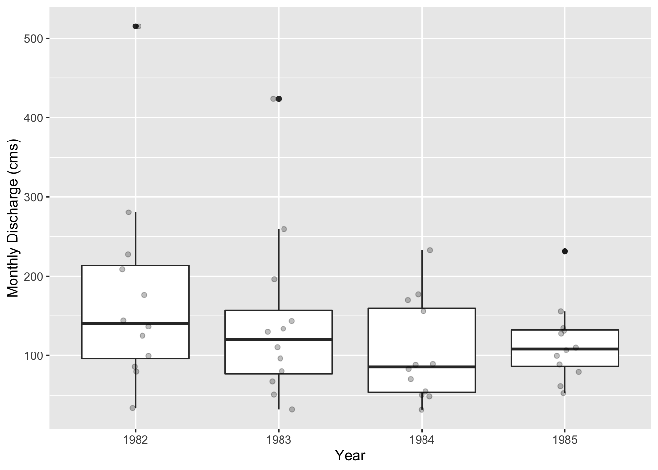
Next, let’s plot the monthly discharge all subbasins versus simulation year.
ggplot(data = output_monthly_rch_test,
       mapping = aes(x = as.factor(YR), y = FLOW_OUTcms, color = as.factor(RCH))) +
  geom_jitter(alpha = 0.25, width = 0.1) +
  facet_wrap(~RCH, ncol = 7) +
  xlab("Year") +
  ylab("Monthly Discharge (cms)") +
  scale_color_discrete(name = "Subbasin ID") +
  theme(axis.text.x = element_text(angle = 90, hjust = 1))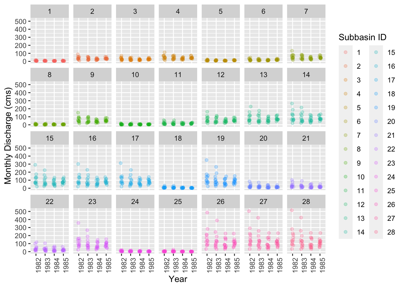
Last, we’ll plot the range of monthly discharge for all subbasins versus month.
ggplot(data = output_monthly_rch_test, mapping = aes(x = as.factor(MO), y = FLOW_OUTcms)) +
  geom_boxplot() +
  geom_jitter(alpha = 0.25, width = 0.1) +
  xlab("Month") +
  ylab("Monthly Discharge (cms)")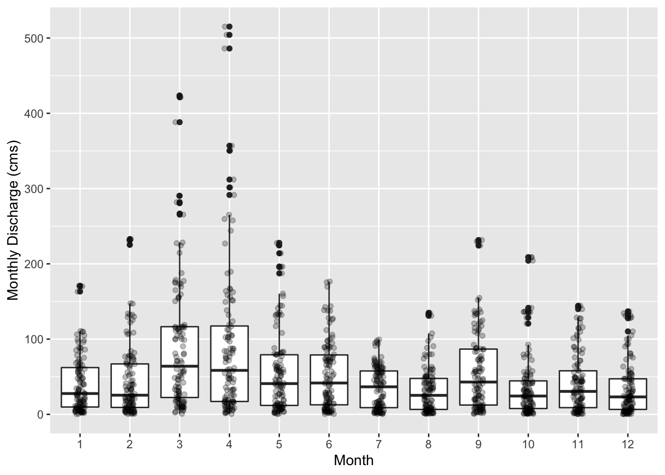
Some other thoughts that I wanted to mention before signing off:
- I think using R to tidy up SWAT outputs is a great way to introduce principles of reproducible to your hydrology data analysis workflows. You can do this by saving the functions above in scripts. If you want to take it a step further you can save the functions to their own R script; where the name of the script is the same as the function name. For example, the code for the
tidy_daily_rch_file()function should be saved totidy_daily_rch_file.R. You can then load this file into your workspace usingload("...tidy_daily_rch_file.R")and use it after loading. - When tidying up the monthly SWAT outputs, I used a for loop but I’m sure there are other more efficient ways of doing this. Maybe using
tidyr::fill()orpurrr::map()? I’ll keep working on this. - Above, I mentioned saving the yearly summary data in a separate data frame and running QA/QC on this with the newly tidied monthly data. This is something I’d like to do eventually.
P.S. Please feel free to use the functions above for your own SWAT output tidying and analysis! Please contact me on Twitter or any other method here if you find any mistakes, have suggestions, or know of any other SWAT data analysis resources for R.